SOLIDIFY · THE SCIENCE

what the instrument actually solves, why it looks like real metallography, and where the model's honesty ends

1 · THE MODEL

SOLIDIFY integrates the Kobayashi (1993) anisotropic phase-field model for an undercooled melt, extended to many grains and a dilute solute. Two coupled fields live on every cell of a 512²–2048² grid: an order parameter φ (0 = liquid, 1 = solid) and a temperature T, with a solute concentration c and a solidification-age channel alongside.

τ ∂φ/∂t = ∇·(ε² ∇φ) + anisotropy terms + φ(1−φ)(φ − ½ + m)

interface relaxation: surface energy vs. thermodynamic driving force

ε(θ) = ε̄ (1 + δ cos j(θ − θ₀)) · m(T, c) = (α/π) atan(γ(1 − m_Lc − T))

j-fold surface-energy anisotropy (j = 4 cubic, 6 hexagonal); driving force from local undercooling, depressed by solute

∂T/∂t = ∇²T + K ∂φ/∂t · ∂c/∂t = ∇·(D(φ)∇c) + (1−k) c ∂φ/∂t

heat diffusion with latent-heat release; solute diffusion with interface rejection (partition coefficient k)

Everything you see follows from these lines. There is no scripted behaviour: no drawn arms, no prebaked snowflakes, no particle effects.

2 · WHY DENDRITES HAPPEN

A flat solidification front in an undercooled melt is unstable: any bump reaches into colder liquid, dumps its latent heat faster, and grows faster still — the Mullins–Sekerka instability. Latent heat (the K ∂φ/∂t term) makes each growing tip warm its own surroundings, so growth self-limits and selects a tip radius; the anisotropy ε(θ) breaks the symmetry so arms lock onto crystal axes. Four-fold anisotropy gives the classic metal dendrite; switch j to 6 and the same equations grow a snowflake, because ice is hexagonal. Interface noise seeds the side-branches, exactly as thermal noise does in reality.

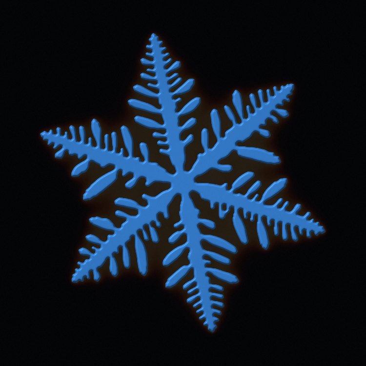
With the anisotropy turned nearly off the model grows seaweed (dense-branching morphology), and with a pulled thermal frame it reproduces columnar growth and the columnar-to-equiaxed transition — all canonical, all emergent.

3 · MANY GRAINS AND TWINS

Each nucleus carries its own crystallographic orientation θ₀ in a grain-ID field that propagates just ahead of the moving front: a newly solidifying cell adopts the identity of its most-solid neighbour. Where two fronts meet, growth stops and a grain boundary is frozen in — no extra model terms. The ASTM E112 grain number shown in the HUD is computed from per-grain pixel counts reduced on the GPU.

Twinning: with a set twin rate, a claim at the growth front occasionally spawns a new domain rotated by π/j — the maximal-misorientation 2D analog of a coherent twin. The twin must then out-grow its parent to survive, which is exactly the competition that selects feathery twinned grains in aluminum DC casting. Two 6-fold seeds locked at 30° grow the rare 12-branched snowflake. Twin boundaries etch faint in the micrograph lens, as coherent boundaries do under a real etchant.

4 · THE ALLOY CHEMISTRY

The solute field implements a Warren–Boettinger-type dilute alloy: the growing solid rejects solute (partition coefficient k < 1), which piles up ahead of the front and lowers the local melting point — constitutional undercooling, the engine of most real dendrites. The rejected solute freezes into the last liquid between the arms as microsegregation, which the XRAY lens renders the way synchrotron radiographs show it.

The alloy composer works in real chemistry. Each element carries approximate textbook dilute-limit binary coefficients (liquidus slope m in K/wt%, partition k). In the dilute limit these superpose:

ΔT_L = Σ m_ic_i · Q = Σ m_ic_i(k_i − 1)

liquidus shift and growth restriction factor — the two numbers that control solidification

Q is the industry-standard growth restriction factor (Easton & StJohn): it measures how strongly a composition slows crystal growth, and it predicts grain refinement. The composer collapses your mix onto the model's single pseudo-binary solute field so that ΔT_L and Q are preserved (k_eff = 1 − Q/|ΔT_L|, the m·c-weighted mean partition), and labels every clamp it has to make.

A RESULT THAT WAS MEASURED WRONG TWICE

Before v4.0 this page reported a clean demonstration: under identical nucleation (a fixed 12 seeds/s rain) and cooling, grain-refined A356+TiB froze into 369 grains while nearly-pure Al–1Zn gave 46 coarse ones. Under the site model that comparison inverted — the lean alloy came out finer — and v4.0 withdrew the claim. v5.0 went back to it and found that the inversion was an artefact too. Two flaws, and neither is physics:

Equal bath temperature is not equal undercooling. A356's liquidus sits at 0.821 where the lean alloy's is 0.993, so at a common start temperature the refined charge began above its own liquidus and could not nucleate at all until it had cooled further. Equal time is not equal progress. Growth restriction left the refined charge with 25× less solid at the moment of comparison (f_s 0.004 vs 0.106) — and grain count is counted on solid that exists.

Control both — start each charge at the same undercooling below its own liquidus, read both at the same solid fraction — and the honest answer is that the two alloys come out the same within noise. Across four independent runs at two inoculant charges the grain counts agree to better than 8 % (1434/1380, 1431/1445, 305/313, 351/327). Growth restriction is unmistakably present — the refined charge takes about twice as long to reach 20 % solid — but at these site densities it does not translate into a finer grain count. Neither the original claim nor its inversion survives a controlled comparison.

One further caution, recorded because it nearly became a third wrong answer. An early v5.0 measurement appeared to show the textbook mechanism — the slower alloy recalescing less, holding its undercooling, and firing every one of its 3000 sites against the lean charge's 1640. It did not reproduce. The harness advances the solver against wall-clock frames, and a GPU-backpressure guard skips frames unpredictably, so the two casts had not received the same amount of physics. Site-firing counts from this harness are not a controlled variable; grain count at matched solid fraction is, which is why that is what the suite asserts (REFINE-FAIR). Settling the mechanism needs a solver that can be stepped a fixed number of substeps regardless of frame pacing, which this one cannot yet do.

The composer's reported chemistry — ΔT_L, Q, k_eff — is computed from the textbook coefficients throughout. Its conversion into the solver's units was itself wrong until v5.0: it used a flat 100 K per dimensionless degree for every metal, where the model's own factor is (L/c_p)/K — about 249 K for aluminium.

The ANALYZE section adds foundry instruments: a cooling-curve probe (a thermal-analysis cup test — recalescence shows as the dip-and-rise), a Scheil overlay comparing the analytic Scheil path T(f_s) = 1 − m·c₀(1−f_s)^k−1 against the measured interface temperature, and an SDAS ruler that measures secondary dendrite arm spacing by linear intercept, the same way a metallographer does it.

5 · NUMERICS AND THE GPU

Explicit Euler on a uniform grid, dimensionless units, dt held inside the stable envelope of the scheme; every UI slider range is clamped so instability is unreachable.
Compact 9-point Laplacians. The naive divergence-of-central-differences builds an effective 2Δx Laplacian that decouples the two checkerboard sublattices and shreds the interface. SOLIDIFY uses the compact 9-point stencil plus a flux texture carrying the anisotropy terms (εε′φ_x, εε′φ_y, ε²), which keeps the front clean.
All WGSL compute. Two passes per substep (flux, update) over ping-pong storage textures, roughly a billion cell-updates per second on a mid-range discrete GPU.
Backpressure. One command submission per frame and a GPU-fence in-flight counter: slow devices throttle gracefully instead of freezing the tab.
GPU statistics. Fraction solid, interface undercooling, per-grain areas (atomic counts → ASTM G), and the cooling-curve probe all come from a single reduction pass.

6 · THE THIRD DIMENSION

The TRUE 3D switch replaces the 2D grid with a full volumetric solver — up to 192³ ≈ 7.1 million voxels stepping the same Kobayashi equations in three dimensions. Surface-energy anisotropy becomes a function of the interface normal n̂ in each grain's own crystal frame (per-grain quaternions carry the orientation):

a(n̂) = 1 + δ(4Σn̂′ᵢ⁴ − 3) · a(n̂) = 1 + δ₆K₆(n̂′) − δ_zn̂′_z²

cubic ⟨100⟩ and hexagonal (basal K₆ + c-axis penalty) anisotropies — δ_z > 0 grows plates, < 0 grows needles

The volume is drawn by raymarching: a ray per pixel steps the φ field, refines the crossing by bisection, and shades the iso-surface with central-difference normals — nine lenses, from incandescent MELT to a volumetric NEON dark-field. The section plane (free depth, tilt and turn, CT sweep) is honest serial sectioning: the STEREOLOGY panel measures grain size on that plane and against the true 3D census, showing the classic section-plane underestimate that stereology exists to correct.

Shrinkage porosity is modelled by feed-path tracking: a flood fill from the riser (top face) marks liquid that can still be fed; liquid that solidifies while cut off becomes a pore, which x-rays dark in the FIELD lens exactly as casting radiography finds it. The flood honours the mould walls — a wall voxel is unconditionally excluded from the feed path every pass, so a chamber sealed behind a partition can never be reached by metal that never crossed it. At every freezing voxel the instrument also records the Niyama criterion Ny = |∇T|/√Ṫ — the foundry's standard porosity-risk index — and can paint it on the section plane. Numerics: explicit Euler at dt = 0.53·dx²/6 (the 3D stability bound), two compute passes per substep over ping-pong 3D storage textures, and 57 bytes of VRAM per voxel across seven textures — ~403 MB at 192³, with an out-of-memory ladder down through 160³, 128³ and 96³ (~50 MB) for smaller GPUs, every rung of it selectable from the ENGINE row.

The volume now carries the whole instrument. The dilute-alloy solute field runs in 3D (a lazily-allocated ping-pong texture pair — the composer's chemistry included), Bridgman growth pulls a thermal gradient up the z-axis, and a steerable laser welds the top surface with Beer–Lambert depth absorption. Growth twins nucleate at the moving front in true Σ3 registry — 60° about a parent ⟨111⟩, spawned on the GPU inside the grain-claiming pass — and the "forbidden" 5-fold symmetry gets its honest 3D answer: icosahedral interface energy built on the six 5-fold axes, growing twelve-lobed quasicrystal shapes. A cusped {100} energy grows genuinely faceted crystals. The one 3D-only scenario is the single-crystal grain selector: a helical "pigtail" channel mask under the Bridgman pull — dozens of chill-floor grains race in, exactly one orientation exits into the blade cavity, which is how real turbine-blade single crystals are actually made. The foundry instruments follow: the cooling-curve probe (ctrl-tap any voxel), the Scheil overlay, an SDAS ruler that measures λ₂ along any dragged line through the volume, and a stereographic pole figure beside the IPF map. The lab's mould is a rasterized geometry library — shell, plate, step, wedge — sharing one voxel-mask entry point regardless of shape. The step block is the classic foundry teaching casting: four section thicknesses fed from one common pour, each freezing at its own rate purely from wall-conduction geometry (no per-section parameter), and each measurable independently by the lab's own per-section census.

7 · NUCLEATION, AND THE LAB

Earlier versions of this instrument let you set the undercooling, the cooling rate and a nucleation rate in nuclei per second. That last slider was wrong, and a reader with a solidification background spotted it immediately: the nucleation rate is not something you set. It is a consequence of the other two. A melt nucleates when it is undercooled enough for the particles it happens to contain to become growth centres, and how deeply it undercools is decided by the competition between the heat you pull out and the latent heat the growing solid gives back.

So the rate is gone, and what remains is what a foundry actually controls — the inoculant. The charge carries n_max potential sites; each one has its own activation undercooling drawn from a Gaussian N(ΔT_N, ΔT_σ), and each fires exactly once, when the melt first gets that cold. This is the Gaussian site-distribution model that Thévoz, Desbiolles and Rappaz introduced for equiaxed casting and that CA-FE codes still use; the "fires once, when the melt first reaches its threshold" rule is the athermal picture Greer's free-growth model makes precise, where a particle's threshold is set by its diameter, ΔT_fg = 4γ/(ΔS_vd).

The consequence is the part worth watching. Sites only activate on a new maximum undercooling, so when recalescence sets in — latent heat warming the melt back up — the sweep stalls and nucleation shuts itself off, exactly as it does in a real casting. Cool the same charge faster and the melt reaches a deeper undercooling before recalescence catches it, so more of the same inoculant activates and the casting comes out finer. That coupling is not scripted anywhere in the code; it falls out, and the instrument's own test suite asserts it: identical charge, cooling rate 0.08 vs 0.45, roughly 300 vs 420 grains.

Lab mode exists because the rest of the instrument is a sandbox — you drag sliders and the melt answers. That is a good way to learn what each term does and a bad model of how the measurement is actually made. In the lab you fix the experiment first: the charge and its inoculant, the atmosphere, the pour superheat, the mould temperature and shape (3D — shell, plate, step or wedge), and a cooling programme (furnace, air, quench, or a soak-then-cool hold). Then you pour it and watch. The solver follows the programme's set-point with Newtonian shell coupling rather than a constant heat sink, which is what lets a hold really hold. At the end you get a report card: the cooling curve read the way a foundry reads a cast cup (T_L, T_N, recalescence, T_S — the thermal-analysis row below says what that extraction can and cannot resolve), the deepest undercooling reached, how much of the inoculant survived the hold and fired, the dissolved-hydrogen ledger, and — since the lab judges as well as measures — the as-cast grain census with its Hall–Petch yield strength, held against a pre-pour spec if you dialled one. The spec is latched at the pour, so moving it after the metal is in the mould cannot rewrite the verdict; a miss points back at this panel, because a finer pour closes it (more inoculant, a shorter hold, a faster programme) where the furnace can only move it further away. Change a physics dial while it is pouring and the card says so — a run with the conditions moved under it is a demonstration, not a measurement. Pour the step block and the card gains a fifth reading: a per-section table, thickness against local d̄ against σ_y, thinnest first — the same census machinery run four times over four regions of the one casting, so the section-thickness effect is a measurement, not an illustration.

8 · THE CALIBRATED SOLVER

Everything above this point is a similarity model. It grows the right shapes for the right reasons, but its interface width and relaxation time are dials — you pick ε̄ and τ, a dendrite appears, and its tip radius is a shape rather than a prediction. The SCALE panel has always said so: the capillary ratio d₀/W reads not defined, because there is no calibrated surface energy anywhere in the Kobayashi model to define it with.

The calibrated solver closes that hole. Karma and Rappel's thin-interface asymptotics relate the phase-field parameters to the two numbers a material actually has — the capillary length d₀ = Γ/ΔT₀ and the diffusivity D — through

d₀ = a₁ W₀ / λ · τ₀ = a₂ λ W₀² / D

a₁ = 5√2/8 = 0.8839 and a₂ = 0.6267 are properties of the chosen interpolation functions, not of any material — and a₂ holds only for h(φ) = φ, which is the heat source this solver uses

so once λ is chosen, W₀ and τ₀ are forced, and with them the physical size of a cell and the physical length of a timestep. Seven dials stop being choices. For Al–4.5Cu that works out to d₀ = 3.2 nm, W₀ = 109 nm and a cell of 0.087 µm, so a 1024² grid is a 89 µm field of view — and the SDAS ruler starts reporting arm spacings a micrograph of the same alloy would give, rather than whatever a declared 1 mm domain happened to imply.

λ is the only knob left, and it is a convergence knob, not a physics one. It sets W₀/d₀: how many capillary lengths wide the diffuse interface is. The asymptotics are exact as that ratio goes to zero, so every quantitative claim has to be shown independent of it — which is a test, not a promise, and it is the test a pretty dendrite cannot pass by looking pretty.

In an alloy the model also carries an anti-trapping current. With no diffusion in the solid, an interface of finite width traps solute it should have rejected; the error is not small and not random, it looks exactly like a larger partition coefficient, and a dendrite grown with it is entirely convincing. The current cancels it. Measured here: with the current on the effective partition coefficient sits on the real k and does not care how wide the interface is; with it off, k_eff runs 24–40 % high and the excess grows with the width.

One consequence arrives for free. Under the calibrated alloy path one dimensionless degree is the alloy's freezing range rather than the latent-heat interval L/c_p, and the app's own shipped nucleation potency — the same dial, unchanged — reads 11 K instead of 37 K. That is the band real castings occupy, reached by fixing the temperature scale rather than by touching the nucleation model.

What it is checked against, and what it measured:

TEST	AGAINST	RESULT
Equilibrium interface profile	tanh of half-width √2·W₀	0.997 W₀
Critical nucleus radius	Gibbs–Thomson R* = d₀/Δ	22.21 vs 22.10 W₀ (0.5 %)
Steady tip velocity V·d₀/D	Karma–Rappel 1998, 2D microscopic solvability at Δ = 0.55, ε₄ = 0.05: 0.0170	0.01679 (1.2 %)
Independence of interface width	same answer at W₀/d₀ = 1.8 → 3.6	6.4 % spread
Parabolic tip radius ρ/d₀	Tong, Beckermann, Karma & Li 2001: 27.6	28.8 (4.4 %)
Effective partition coefficient	the real k, independent of interface width	k_eff = 0.135–0.150 against k = 0.15; 0.186–0.209 with the current off
Solute conservation	flat over 20 000 substeps of growth	1.6×10⁻³

And what it does not fix. The Lewis mismatch is unchanged — one explicit grid at one timestep still cannot carry heat and solute four orders apart, and the alloy path anchors on solute. The calibrated solver is 2D only; the volume still runs the Kobayashi model, and the switch says so rather than appearing and doing nothing. And the thin-interface expansion has a validity bound of its own, τ₀V/W₀ ≲ 0.2, which a deeply undercooled pure melt reaches by λ ≈ 4 — the app reports λ and the ratio it implies so that stays visible.

9 · HEAT TREATMENT — THE SECOND CLOCK

Everything above runs on the solidification clock, and under the calibrated solver a timestep on that clock is of order 10⁻⁷ s. A heat treatment is four hours — about 10¹¹ timesteps — so the phase-field solver can never be integrated through one: not slowly, not on a bigger GPU, not ever. Pretending otherwise would be the category of claim this page exists to rule out. So heat treatment is a separate model on a separate clock. You set a real schedule in °C and hours; every rate law the material shipped with is integrated over that schedule's whole trajectory — Simpson through the ramps, because an Arrhenius rate varies by orders of magnitude across one and charging only the hold under-counts a slow furnace by a measured 31 % — and the integrals become budgets a GPU pass then spends. φ is frozen for the duration, which is what solid state means, so the two clocks never have to be reconciled. No panel ever prints an unlabelled time: sim time is solidification, real hours are the furnace.

There is no process switch. You set an environment — a temperature schedule — and the model reports what happened: grains coarsened this much, solute flattened that much, this thickness of scale grew. "Stress relief" is not a mode; it is what you get when you pick a low temperature and every integral comes back negligible, and the report card says so because the arithmetic said so. This is the same move that deleted the nucleation-rate slider in v4.0: the dependent quantity stops being a dial.

Dⁿ − D₀ⁿ = ∫k(T)·dt · D^m − D₀^m = K_MC·S

two growth laws and two exponents. n is the MATERIAL's, from its sourced coefficients; m is the MODEL's — a measured property of the Monte Carlo Potts pass, like K_MC itself. They meet at the endpoint and nowhere else: the material law says where the grain finishes, the model spends whatever sweeps its own kinetics need to get there, and the trajectory in between is the model's, not the material's

Grain growth is a sublattice Monte Carlo Potts pass on the as-cast grain field, and its two constants are measured, not assumed. Ideal curvature-driven growth is parabolic; a Potts lattice is not — it pins, and its measured exponent comes out m = 2.44 in the plane (three independent casts: 2.38 / 2.44 / 2.61, and this coincides with the canonical Potts result R ∝ t^0.41, measured here rather than adopted) and m = 2.25 in the volume, where all the ingredients differ: 26 neighbours, eight sublattice colours, a cubic lattice with its own pinning geometry. Assuming the textbook m = 2 costs a 4.8× error in the sweep budget — in a number nothing else in the app would have contradicted — which is why the suite makes the two exponents disagree on purpose (HT-SWEEPS) and re-measures K_MC's drift on every run.

Annealing twins appear in the volume, where a Σ3 — 60° about ⟨111⟩ — means something. The data decides who twins: stacking-fault energies were looked up with sources, and the matrix they produce is the teaching point. Copper (78 mJ/m²) and cobalt (≈20) twin; aluminium (166) and nickel (128) refuse with their numbers printed; steel refuses structurally, because it is modelled as BCC δ-ferrite and annealing twins are an austenite phenomenon this solver has no phase for. A twin that forms must also survive its own anneal, and that takes two pieces of real physics: a Σ3 energy cusp at the measured copper ratio (coherent ≈ 24 against general ≈ 625 mJ/m²) and a Σ3 mobility gate — coherent interfaces cannot migrate by single-atom shuffles, which is why twins survive where ordinary boundaries sweep past.

A NUCLEATION MECHANISM THAT WAS BUILT AND MEASURED DEAD, TWICE

The plan's twin-spawn mechanism — a per-cell flip at the migrating boundary, the same idiom the growth twins use — was built exactly as designed and measured dead: 3 of 512 spawned twins survived 300 sweeps, and none survived 450. Adding the mobility gate (true physics) helped by 5× and was still dead. The real killer was geometric: a cell adopting a one-voxel twin pays ~12 neighbours of Σ3 energy where adopting its parent pays ~one — an artificial nucleation barrier no cusp value removes, because a {111} stacking event is sub-grid for a per-cell flip. Real annealing twins are born as plates, and mesoscale models in the literature insert them. So nucleation here is a stamped {111} plate in exact Σ3 registry on a probed boundary, and everything after birth is the pass's own physics. The plate is the one inserted thing — stated here for the same reason the 2D solver does not claim to resolve capillary-length nucleation.

Homogenization is its own pass — masked isotropic diffusion of solute through the solid skeleton at frozen φ — because under the calibrated alloy model the solid diffusivity is exactly zero and there is nothing to reuse. The map from schedule to iterations is exact: iterations = Dt/(cell²·D̃), with Dt the schedule's own Arrhenius integral — no wavelength, no fitted constant — which is why its gate can be an equality test: a seeded eigenmode of the discrete stencil must decay as (1 − 2D̃(1 − cos k))^I, and does, to a relative error of 9·10⁻⁷ in both dimensions with conservation to 10⁻⁷. The continuum answer e^−Dk²t differs from the discrete one by +0.012 % / −0.034 % at the tested modes, and that gap is printed, because it is the model's own discretization error. The cost wall is budgeted honestly: explicit diffusion under the calibrated 0.087 µm cell can demand millions of iterations, so the pass runs what fits and the card reports the delivered fraction of the requested Dt — never silently fewer.

Oxidation and decarburization are analytic card lines, not fields: scale grows as x = √(∫k_p·dt) for every material with a sourced parabolic constant, and steel alone decarburizes as x = 2√(D_Ct), because steel is the one material here whose solute is carbon. The span is the teaching point — aluminium's passive film comes out 2.3 nm after 14.5 h at 520 °C ("aluminium does not scale", made visible) against steel's mill-scale millimetres. Ice and succinonitrile refuse by name: a zero in the constants table means "no constant was looked up", not "0 µm of scale". The scale is deliberately not painted into the fields — T, c and age are the as-cast record, and the card is where the number lives.

Strength rides the grain size. The report card closes with σ_y = σ₀ + k_HP/√d̄ — Hall–Petch on the measured census, before and after — and a verdict against a spec you commit before the run, the way a real heat treatment answers to a drawing requirement. Three limits are printed with the number. It is grain-size strengthening alone: no precipitates, no work hardening — see the aging row below. The d̄ under the root is the census's equivalent diameter (area-equivalent circle in the plane, volume-equivalent sphere in the volume), an O(1) stereological factor from the mean linear intercept the tabulated constants were fitted to. And the µm inside √d̄ stand on the declared resolution — "you set it" is the length anchor's provenance, and the strength inherits it. One consequence is stated rather than hidden: this furnace can only coarsen, and coarser is softer, so a spec above the casting's current strength is unreachable by any schedule. Meeting it takes a finer pour, and the panel says so before you waste the furnace time.

What it is checked against, and what it measured:

TEST	AGAINST	RESULT
Arrhenius integral, hold	closed form	rel. err. 3×10⁻¹⁵
Arrhenius integral, ramp	the same quadrature at 64× the samples (a ramp has no elementary integral)	3×10⁻⁸
2D Potts kinetics (m, K_MC)	its own fit, pinned intercept, transient excluded	m = 2.44 (2.38 / 2.44 / 2.61 across casts), K = 4.79, drift gated at 25 %
3D Potts kinetics (m, K_MC)	same doctrine, measured separately — 26 neighbours, 8 colours	m = 2.25, K = 1.28 (1.8 % spread), drift gated at 15 %
Panel end-to-end (2D)	the material law's endpoint for a 12 h / 520 °C anneal of aluminium	d̄ 14.0 → 48.6 µm vs 50.4 µm — 0.96–1.00 of the law across runs
Homogenization decay	the DISCRETE stencil eigenvalue, exact	9×10⁻⁷ (2D and 3D); continuum gap +0.012 % / −0.034 %, printed
Σ3 twin registry	exact Σ3 against each twin's real volume neighbours	25/26 exact; 22 of 26 alive after 150 further sweeps
σ_y row and spec verdict	Hall–Petch on the same census the gate reads; a spec committed under the as-cast strength	row equals the law to 0.2 MPa; the anneal misses the spec, the stress relief meets its own

And what it does not do. No precipitate aging, no T6: the material table carries no precipitate kinetics — no volume fractions, no coarsening rates — and inventing them to draw a JMAK curve is the one thing this instrument does not do, so the strength row is grain size only and says so. Grain growth here is unpinned — no second-phase particles, no solute drag, no thermal grooving — so a real specimen stalls where this one keeps going. The hold is isothermal by construction: the solver's temperature field is the as-cast record, not the furnace, so the treatment parks the thermal lenses and puts up a banner instead of showing a cold casting labelled 540 °C. And the specimen is finite: grain statistics stop meaning anything when a handful of grains fill the frame, so a schedule whose own law predicts a grain the domain cannot carry is refused with the analytic answer still printed — steel's one-hour anneal at 0.85 T_m says 296 µm, the volume is 188 µm across, and the model declines to pretend otherwise.

10 · WHAT'S QUANTITATIVE, WHAT'S QUALITATIVE

CLAIM	STATUS
Dendrite/seaweed/snowflake morphology, tip selection, side-branching	canonical — matches the published Kobayashi figures
Mullins–Sekerka breakup, CET, columnar growth, weld epitaxy	emergent physics, qualitatively correct
Grain impingement, ASTM E112 grain number, linear-intercept SDAS	measured honestly on a nominal 1 mm domain
Alloy solute field	two solvers, and the app says which is running. The default is a WB-type dilute model, qualitative and not CALPHAD-coupled. The calibrated solver is the Echebarria–Folch–Karma–Plapp dilute binary model with an anti-trapping current, where the partition coefficient is the real one and is independent of the interface width — still dilute-binary and still not CALPHAD-coupled
Composer chemistry (ΔT_L, Q, wt%↔at%)	real dilute-limit values, approximate textbook coefficients
Units	a stated similarity scaling — the solver is dimensionless, and three factors convert it to SI: kelvin per unit, seconds per unit, µm per cell. Only the third is a free choice. Kelvin per unit is forced by the heat equation's own latent coupling, (L/c_p)/K — a real per-material number (≈249 K for aluminium, ≈44 K for water), not the flat ~100 K this row used to claim. Seconds per unit is then forced by whichever diffusivity is transporting. Every panel shows which factor was chosen and which were forced, and the SCALE report names the dimensionless groups the model does not match
Lewis number α/D (the load-bearing mismatch)	not matched, and it cannot be — a real alloy separates heat and solute by four orders of magnitude; one explicit grid at one timestep cannot carry both. With the solute anchor the temperature field diffuses far too slowly, so read it as the imposed macroscopic temperature rather than real heat conduction at this scale. That is the direction a micro-scale casting model errs in anyway, and it is reported rather than hidden
Tip radius, tip velocity, arm spacing	shapes under the default solver, predictions under the calibrated one. Kobayashi has no calibrated surface energy, so there is no length to compare a tip radius against; the calibrated solver derives W₀ from the material's own d₀ and reproduces the published 2D solvability tip velocity to 1.2 % and the parabolic tip radius to 4.4 %
Grain size and arm spacing in µm	measured against the model resolution, which is now the anchor: the domain is n × µm-per-cell wide, not a fixed 1 mm. It was the other way round until v5.0, which meant the same dendrite measured four times larger at 512² than at 2048². Every µm figure printed before that fix is wrong by the grid ratio unless it was taken at the default grid
Dimensionality	2D by default (thin-sample analog) — the TRUE 3D mode solves the full volume, where dendrites genuinely branch out of plane
Porosity + Niyama (3D)	mechanistic, and quantitative for steel only — feed-path flood + solidify-while-unfed rule for the pores; Ny = \|∇T\|/√Ṫ recorded at the moment each voxel freezes, with Ṫ the non-latent environment rate (conduction, the sink, and the imposed scenario's own continuous cooling — the voxel's recalescence is the one deliberate exclusion) and −1 stored where no front ever passed (seed cores, freeze-while-warming) rather than a fabricated safe number. With real units the map converts to K·s^½·mm⁻¹, and for STEEL the section-plane legend judges it against Niyama's own radiographic criterion, 0.775 K^½·s^½·mm⁻¹; every other material keeps a relative map, because that threshold is steel radiography and this instrument's aluminium porosity is Sievert hydrogen, not shrinkage. The printed value inherits the scale layer's anchors — the legend names which clock it is standing on
Hot tearing	a timing index, not a stress prediction — the lab card prints the Clyne–Davies cracking susceptibility CSC = t_v/t_r off the pour's own recorded f_s(t) (vulnerable 0.90→0.99, relieving 0.40→0.90). The index is defined on a local volume element and this record is the global open-cavity fraction, so on a directional front it degenerates toward a geometry constant — the card says so. The RDG criterion the roadmap once named needs a transverse strain rate and a Darcy feeding term this solver does not carry, and no number is printed that pretends otherwise
Gas porosity from dissolved hydrogen (the lab)	Sievert's law with real solubility, a proxy for the rest. A melt dissolves hydrogen as C = S·√p, and the solubility collapses on freezing — liquid aluminium holds ~19× the solid, so the rejected difference feeds gas pores. Real: the Ransley–Neufeld solubilities (Al liquid ≈0.69, solid ≈0.036 cm³/100 g at 1 atm), the √p pressure dependence, and the liquid→solid drop that drives it. Proxy: how much hydrogen each atmosphere presents (air humid → charged, cover gas → residual, vacuum → degassed — an ordering, not measured partial pressures) and the map from rejected hydrogen to the pore field. A material with no solubility data refuses gas porosity by name. This replaced a flat "+0.1 in air" bias; the pore field itself is 3D
Grain selector (3D)	geometric — real selector physics (columnar competition through a constriction); the pigtail shape is procedural, not a specific foundry's
Mould geometry (3D)	exact rasterization, real conduction, teaching proportions — shell/plate/step/wedge are deterministic integer voxel math, gated bit-exact against an independent GPU mask readback; once poured, the mould wall is a real cold boundary condition and section-thickness effects (the step block's whole point) emerge from conduction toward it, not from a per-section parameter. The four step-block thicknesses are a teaching proportion, not a measured specimen. A grain spanning two sections is counted in both — the same thing a metallographer's per-field measurement does
Icosahedral quasicrystal (3D)	interface-energy symmetry only — the aperiodic lattice itself is beyond a phase-field order parameter
Melt glow per material	display only — incandescence scaled to each metal's freezing point
Nucleation site model (n_max, ΔT_N, ΔT_σ)	mechanistic, not derived — the Rappaz/Greer structure (Gaussian activation undercoolings, fire-once, recalescence ratchet) with thresholds chosen to be watchable, not computed from interfacial energies. Real inoculated aluminium activates within a few kelvin of the liquidus; here the distribution is stretched across the range you can actually drive
Where the undercooling is measured	global sweep, local firing — the ratchet reads the mean melt temperature, so in a strong gradient a site can be spent while its own neighbourhood is still hot; whether it actually nucleates is then checked cell-by-cell against the local liquidus, and in the volume that liquidus is the nominal one (the 3D stamp pass carries no solute field)
Atmosphere (air / argon / vacuum)	cleanliness proxy — NOT a nucleation control. Atmosphere does not change how readily bulk liquid nucleates. What it changes in reality is oxidation: a melt poured in air entrains oxide films, which are wall and defect features. Here air adds shallow-threshold sites in the wall band and, through the hydrogen it carries, drives gas porosity by Sievert's law (see the gas-porosity row); nothing else. Bifilms form even under cover gas, so "argon" is cleaner, not clean
Cooling programmes (furnace / air / quench)	Newtonian shell coupling in dimensionless temperature — the ordering of the three (roughly 0.2, 1–10 and 100+ K/s in a real shop) is preserved; the absolute rates are not
Cooling-curve thermal analysis (the lab report card)	a real extraction, read honestly. The report card analyses the recorded cooling curve the way a foundry reads a cast cup: liquidus arrest T_L, nucleation nadir T_N and recalescence ΔT_r, solidus T_S, freezing range, local solidification time and the liquid cooling rate — landmarks located from a time-based (not index-based) windowed derivative, and any it cannot resolve are shown as unresolved, never filled in. Solid fraction is also reconstructed from a single-sided Newtonian zero curve and printed against the solver's measured census, so the number you see is the method's own error. Two honest limits: the "thermocouple" is the mean temperature of the remaining liquid, not a fixed probe — so part of any recalescence shown is a selection effect as cold cells leave the average — and the record ends at the solidus, because past it there is no liquid to read and the two-sided Newtonian baseline a full analysis wants is simply absent
Pour superheat, mould temperature	qualitative boundary conditions — superheat is a real thermal load and the mould is a real cold boundary. (Whether the refiner is faded by high superheat specifically is not separated out here; fade is driven by hold time — see the next row.)
Grain-refiner fade (hold before pour)	an empirical time law, labelled as one. Hold an inoculated charge above its liquidus and it loses effective nucleant sites: the refining particles (TiB₂, Al₃Ti in the Al–Ti–B system) are denser than the melt and settle out — faster than Stokes' law alone, because they agglomerate and catch on oxide films. The lab models this as a short potent plateau then an exponential decay to a residual floor, with most of the loss inside the first ~30 min (the settling literature) and exactly no fade at zero hold, so nothing shipped earlier moves. The timescale is the Al–Ti–B holding picture applied to whatever inoculant you set — it is not derived from a specific particle-size distribution
Stirring, convection, melt flow	not modelled at all — grain multiplication by dendrite fragmentation is a real and important refining mechanism, and it needs a flow field this solver does not have
Solid-state grain growth (HEAT TREAT)	endpoint from the material's sourced law, trajectory from measured Potts kinetics — Dⁿ − D₀ⁿ = ∫k·dt says where the grain finishes; the model's own (m, K_MC) pair, measured per dimension, spends the sweeps. Unpinned: no particles, no solute drag, so a real specimen stalls where this one keeps going
Annealing twins (3D)	real crystallography, inserted birth — exact Σ3 registry, survival by a measured-ratio energy cusp plus a mobility gate; but the nucleus is a stamped {111} plate, because a per-cell spawn was built twice and measured dead — a stacking event is sub-grid for a Potts flip. Who twins is decided by sourced stacking-fault energies (Murr 1975)
Homogenization	exact, and gated as an equality — masked diffusion at frozen φ whose iteration count is the schedule's own Dt product, no fitted constant; the discrete-vs-continuum gap is printed as the model's own discretization error, and the delivered fraction of a budget-capped soak is reported, never silently fewer
Oxide scale, decarburization	analytic card lines — parabolic laws over the whole schedule from sourced constants; never painted into the fields, which are the as-cast record. Ice and SCN refuse by name rather than draw a confident 0 µm
Yield strength σ_y (Hall–Petch)	grain-size term only — σ₀ + k_HP/√d̄ on the measured census, no precipitates, no work hardening; d̄ is the equivalent diameter (an O(1) factor from E112's mean intercept), and the µm under the root are the declared resolution. The spec verdict judges this number and names these limits — on both cards: the furnace's post-treatment verdict and the lab's as-cast one share one d̄ definition, one formatter and one printed-precision rule, so a casting can never carry two strengths
Precipitate aging / T6	not modelled at all — the material table has no precipitate kinetics, and a JMAK curve drawn from invented per-material numbers would be a prediction this instrument has no right to make

The rule throughout: anything the instrument displays as a number is computed, and anything that is a stylistic choice is labelled as one.

11 · REFERENCES

R. Kobayashi, “Modeling and numerical simulations of dendritic crystal growth,” Physica D 63 (1993) 410–423.
Ph. Thévoz, J.L. Desbiolles & M. Rappaz, “Modeling of equiaxed microstructure formation in casting,” Metall. Trans. A 20 (1989) 311–322 — the Gaussian site-distribution nucleation model.
Ch.-A. Gandin & M. Rappaz, “A coupled finite element–cellular automaton model for the prediction of dendritic grain structures in solidification processes,” Acta Metall. Mater. 42 (1994) 2233–2246.
A.L. Greer, A.M. Bunn, A. Tronche, P.V. Evans & D.J. Bristow, “Modelling of inoculation of metallic melts: application to grain refinement of aluminium by Al–Ti–B,” Acta Mater. 48 (2000) 2823–2835 — free growth, and why only a small fraction of particles ever become grains.
W. Oldfield, “A quantitative approach to casting solidification: freezing of cast iron,” Trans. ASM 59 (1966) 945–961 — nucleation count as a function of undercooling.
J.A. Dantzig & M. Rappaz, Solidification, EPFL Press (2009) — recalescence and the heat-extraction / latent-heat competition that sets grain density.
E. Fras, W. Kapturkiewicz, A. Burbielko & H.F. Lopez, “A new concept in thermal analysis of castings,” AFS Trans. 101 (1993) 505–511 — the Newtonian zero-curve method the lab report card inverts for solid fraction.
D.M. Stefanescu, “Thermal analysis — theory and applications in metalcasting,” Int. J. Metalcast. 9 (2015) 7–22 — cooling-curve landmark extraction (T_L, T_N, recalescence, T_S).
J. Campbell, Castings, Butterworth-Heinemann (2003) — entrained oxide films (bifilms) and what melt atmosphere actually governs.
A. Karma & W.-J. Rappel, “Quantitative phase-field modeling of dendritic growth in two and three dimensions,” Phys. Rev. E 57 (1998) 4323–4349.
B. Echebarria, R. Folch, A. Karma & M. Plapp, “Quantitative phase-field model of alloy solidification,” Phys. Rev. E 70 (2004) 061604 — the dilute binary model and the anti-trapping current.
A. Karma, “Phase-field formulation for quantitative modeling of alloy solidification,” Phys. Rev. Lett. 87 (2001) 115701.
X. Tong, C. Beckermann, A. Karma & Q. Li, “Phase-field simulations of dendritic crystal growth in a forced flow,” Phys. Rev. E 63 (2001) 061601 — the 2D tip-radius benchmark this app is checked against.
E. Niyama, T. Uchida, M. Morikawa & S. Saito, “A method of shrinkage prediction and its application to steel casting practice,” AFS Int. Cast Metals J. 7 (1982) 52–63 — the Niyama criterion, and the steel radiographic threshold (1.0 (°C·min)^½·cm⁻¹ = 0.775 K^½·s^½·mm⁻¹) the section-plane legend judges against.
T. W. Clyne & G. J. Davies, “The influence of composition on solidification cracking susceptibility in binary alloy systems,” Br. Foundryman 74 (1981) 65–73 — the cracking-susceptibility timing ratio the lab card prints.
J.A. Warren & W.J. Boettinger, “Prediction of dendritic growth and microsegregation patterns in a binary alloy using the phase-field method,” Acta Metall. Mater. 43 (1995) 689–703.
W.W. Mullins & R.F. Sekerka, “Stability of a planar interface during solidification of a dilute binary alloy,” J. Appl. Phys. 35 (1964) 444–451.
M. Easton & D. StJohn, “Grain refinement of aluminum alloys,” Metall. Mater. Trans. A 30 (1999) 1613–1633 — the growth restriction factor Q, and refiner behaviour.
“Grain refiner settling and its effect on the melt quality of aluminium casting alloys,” Materials 15 (2022) 7679 — settling of TiB₂/Al₃Ti particles faster than Stokes' law, the basis for the fade time law.
C.E. Ransley & H. Neufeld, “The solubility of hydrogen in liquid and solid aluminium,” J. Inst. Metals 74 (1948) 599–620 — the liquid and solid hydrogen solubilities behind the Sievert gas-porosity model.
W. Kurz & D.J. Fisher, Fundamentals of Solidification, Trans Tech (1998) — source style for the dilute binary coefficients.
E. Scheil, “Bemerkungen zur Schichtkristallbildung,” Z. Metallkd. 34 (1942) 70–72.
J.E. Burke & D. Turnbull, “Recrystallization and grain growth,” Prog. Met. Phys. 3 (1952) 220–292 — curvature-driven parabolic grain growth, the ideal the Potts pass is measured against.
M.P. Anderson, D.J. Srolovitz, G.S. Grest & P.S. Sahni, “Computer simulation of grain growth — I. Kinetics,” Acta Metall. 32 (1984) 783–791 — the Monte Carlo Potts model, and why its measured exponent sits below the ideal ½.
L.E. Murr, Interfacial Phenomena in Metals and Alloys, Addison-Wesley (1975) — the stacking-fault and twin-boundary energy compilation behind the annealing-twin matrix.
E.O. Hall, “The deformation and ageing of mild steel: III — discussion of results,” Proc. Phys. Soc. B 64 (1951) 747–753.
N.J. Petch, “The cleavage strength of polycrystals,” J. Iron Steel Inst. 174 (1953) 25–28 — with Hall above, the σ₀ + k/√d law the report card's strength row uses.
C. Wagner, “Beitrag zur Theorie des Anlaufvorgangs,” Z. Phys. Chem. B 21 (1933) 25–41 — the parabolic oxidation law behind the scale and decarburization card lines.
ASTM E112, Standard Test Methods for Determining Average Grain Size.